System Dynamics

System Dynamics CPT Rick Mard August 30, 2017

1 Introduction

This tutorial is intended to introduce system dynamics modeling concepts and techniques using the R programming language. The concepts and techniques presented herewithin are simple examples designed for the reader to follow along using R Studio. Therefore, both R and R Studio are suggested in order to fully benefit from the proceeding tutorial.

1.1 Packages

The following packages are used throughout the tutorial. The deSolve package is primarily used to calculate the differential equations and numerical integration. Other required packages include ggplot2, gridextra, plyr, magrittr, and grid. These packages support visualizations, data frame manipulation, and pipe operators.

library(deSolve) #supports numerical integration using a range of numerical methods
library(ggplot2) #supports visualization of layered graphics
library(gridExtra) #supports visualization of multiple plots & graphs
library(plyr) #supports data frame merging
library(magrittr) #supports pipe function
library(grid) #supports additional graphing capability

2 System Dynamics Background

System dynamics is a methodology applicable to modeling factors of a convoluted system of interdependent factors such as the one presented in this tutorial. Jay Forrester discovered system dynamics following his work with management at General Electric and with radar systems for the US Navy. He blended the complexities of social systems with physical systems at the recently established School of Management at the Massachusetts Institute of Technology, or MIT (Forrester 1968). Forrester describes systems as

a grouping of parts that operate together for a common purpose (System Dynamics Society 2017).

The DoD operates in a hierarchical manner with information and knowledge controlled by classification and necessity. Relatedly, Forrester informs that “without an organizing structure, knowledge is a mere collection of observations, practices and conflicting incidents” (System Dynamics Society 2017). To arrive at solutions for strategic and operational planning efforts, systems that define the intricacies and relationships within the operational environment are necessary.

2.1 Models

A system dynamics model contains causal loops that identify the feedback of interactions between elements of a system. These causal loops are usually converted to ‘stocks’ and ‘flows’. Stocks represent elements with capacities that change over time. Flows define the rate at which a stock can change.

Stock and flow diagrams display the interactions between elements in the system so information can be traced throughout. Linear and/or continuous equations in time are applied to the system flows before initializing the system with appropriate stock levels based on expert input, previous research, or analyses (Duggan 2016).

2.2 Stocks & Flows

A stock is the foundation of any system (Meadows 2008), and stocks and flows are the building blocks of system dynamics models. They characterize the state of the system under study, as well as providing the information upon which decisions and actions are based (Sterman 2000). Stocks can only change through their flows, which are the quantities added to (inflow), or subtracted from (outflow), a stock over time (Duggan 2016)

Stock and flow model of customers

Stock and flow model of customers

2.3 Feedback

Feedback is a critical element of system dynamics (Lane 2006), and identifying feedback loops in social systems is an important part of model building. Meadows (2008) describes a feedback loop as:

A closed chain of causal connections from a stock, through a set of decisions or rules or physical laws or actions that are dependent on the level of the stock, and back again through a flow to change the stock.

A feedback loop is a chain of circular causal links, where the level of a stock influences a flow, which in turn will change the stock. The stock can influence the flow directly, or that influence could be determined through a series of intermediate auxiliary variables. Feedback processes are present in many systems. Earlier, when discussing stocks and flows, a warehouse example was presented. This can be examined in more detail to uncover a feedback process in operation (Duggan 2016).

3 deSolve Package

R’s deSolve package solves initial value problems written as ordinary differential equations (ODE), differential algebraic equations (DAE), and partial differential equations (PDE) Soetaert et al. (2010). For system dynamics models, the ODE solver in deSolve is used. The key requirement is that system dynamics modelers implement the model equations in a function, and this function is called by deSolve (Duggan 2016). First, we initialize the simulation time constants and create simluation time vector using seq():

# Set time period and step
START <- 2020
FINISH <- 2050
STEP <- 0.25
simtime <- seq(START, FINISH, by = STEP)

head(simtime)

## [1] 2020.00 2020.25 2020.50 2020.75 2021.00 2021.25

tail(simtime)

## [1] 2048.75 2049.00 2049.25 2049.50 2049.75 2050.00

The model vectors include stocks and its initial value and auxs, which are the exogeneous parameters.

# Set stock capacity, growth and decline rates
stocks <- c(sCustomers = 10000)
auxs <- c(aGrowthFraction = 0.08, aDeclineFraction = 0.03)

A function is created to execute the equations for simulation time, current stock vector, and model parameters. These are stored with as.list() for access. These are flows for recruits and losses along with net flow, a derivative. The data frame ‘o’ is defined to allow the deSolve package function ode to solve the previous equations. The resulting outputs include summary statistics for visualizations.

# Create the function and returns a list
model <- function(time, stocks, auxs){
  with(as.list(c(stocks, auxs)), {
    fRecruits <- sCustomers * aGrowthFraction
    fLosses <- sCustomers * aDeclineFraction
    dC_dt <- fRecruits - fLosses
    return (list(c(dC_dt),
                 Recruits = fRecruits, Losses = fLosses,
                 GF = aGrowthFraction, DF = aDeclineFraction))
  }) 
}

# Create the data frame using the `ode` function
o <- data.frame(ode(y = stocks, times = simtime, func = model,
                    parms = auxs, method = "euler"))

head(o)

##      time sCustomers Recruits   Losses   GF   DF
## 1 2020.00   10000.00 800.0000 300.0000 0.08 0.03
## 2 2020.25   10125.00 810.0000 303.7500 0.08 0.03
## 3 2020.50   10251.56 820.1250 307.5469 0.08 0.03
## 4 2020.75   10379.71 830.3766 311.3912 0.08 0.03
## 5 2021.00   10509.45 840.7563 315.2836 0.08 0.03
## 6 2021.25   10640.82 851.2657 319.2246 0.08 0.03

tail(o)

##        time sCustomers Recruits   Losses   GF   DF
## 116 2048.75   41728.11 3338.248 1251.843 0.08 0.03
## 117 2049.00   42249.71 3379.977 1267.491 0.08 0.03
## 118 2049.25   42777.83 3422.226 1283.335 0.08 0.03
## 119 2049.50   43312.55 3465.004 1299.377 0.08 0.03
## 120 2049.75   43853.96 3508.317 1315.619 0.08 0.03
## 121 2050.00   44402.13 3552.171 1332.064 0.08 0.03

summary(o[,-c(1, 5, 6)])

##    sCustomers       Recruits        Losses      
##  Min.   :10000   Min.   : 800   Min.   : 300.0  
##  1st Qu.:14516   1st Qu.:1161   1st Qu.: 435.5  
##  Median :21072   Median :1686   Median : 632.2  
##  Mean   :23112   Mean   :1849   Mean   : 693.4  
##  3rd Qu.:30588   3rd Qu.:2447   3rd Qu.: 917.6  
##  Max.   :44402   Max.   :3552   Max.   :1332.1

In the graph below the number of customers are a result of the differential equation of recruits and losses defined in the function model above.

Plot the output

o %>% 
  ggplot() +
  geom_line(aes(time, o$sCustomers), colour = "blue") +
  geom_point(aes(time, o$sCustomers), colour = "blue") +
  scale_y_continuous() +
  ylab("Customers") +
  xlab("Year") +
  ggtitle("Customers Over Time", subtitle = "2020 - 2050")

## Warning: Use of `o$sCustomers` is discouraged.
## ℹ Use `sCustomers` instead.
## Use of `o$sCustomers` is discouraged.
## ℹ Use `sCustomers` instead.

4 Limits to Growth

It is necessary to introduce a formulation method before presenting the limits to growth model. Formulation models allows developers to create equations robust enough to model the effect of a variable on another. They are useful for a wide variety of system dynamics models especially those with influencing stocks in different systems.

We begin with modeling causal relationships using effects. This is defined as

\[Y=Y∗∗Effect(X1onY)∗...∗Effect(XnonY)\]

where, based on the assumptions:

• \(Y\) = dependent variable of a causal relationship and is a function of n independent variables (X1,X2,…,Xn)

• \(Y∗\) = reference value, which is the normal value the variable Y takes on. This reference value is multiplied by a sequence of effect functions that are calculated based on the normalized ratio of input term \((Xi/X∗i)\) where \(X∗i\) is the reference input value, and \(Xi\) is the actual input value.

The effect function has the normalized ratio (X/X∗) on its x-axis, and always contains the point (1, 1). This point (1, 1) is important for the following reason: if x equals its reference value X∗ , then the effect function will be 1, and therefore y will then equal its reference value Y∗ .

4.1 Example

Using a single X value, \[GrowthRate=RefGrowthRate∗EffectofAvailabilityonGrowthRate\]

\[EffectofAvailabilityonGrowthRate=f(AvailabilityRefAvailability)\]

• RefGrowthRate=0.10
• RefAvailability=1.0

Relationship between availability and effect on growth rate Relationship between availability and effect on growth rate

The linear relationship between availability and growth rate in the two extreme cases above are either,

• Availability = 1, Effect = 1, so growth rate is maximized
• Availability = 0, Effect = 0, since there are no resources, therefore growth rate is zero

which keeps the model simple and follows the slope-intercept equation of \(y=mx+c\) . The effect equation can be modified from above.

\[EffectofAvailabilityonGrowthRate=AvailabilityRefAvailability\]

Growth rate depends on the value of availability through the variable effect as seen in the table below.

Ref availability	Availability	Effect of availability on growth rate	Ref growth rate
1.0	1.0	1.0	0.10
1.0	0.5	0.5	0.10
1.0	0.0	0.0	0.10

4.2 S-Shaped Growth

From the previous model, a limiting factor is added as a balancing loop to counter growth as in the model below

4.2.1 Define Variables

A one-stock model of limits to growth

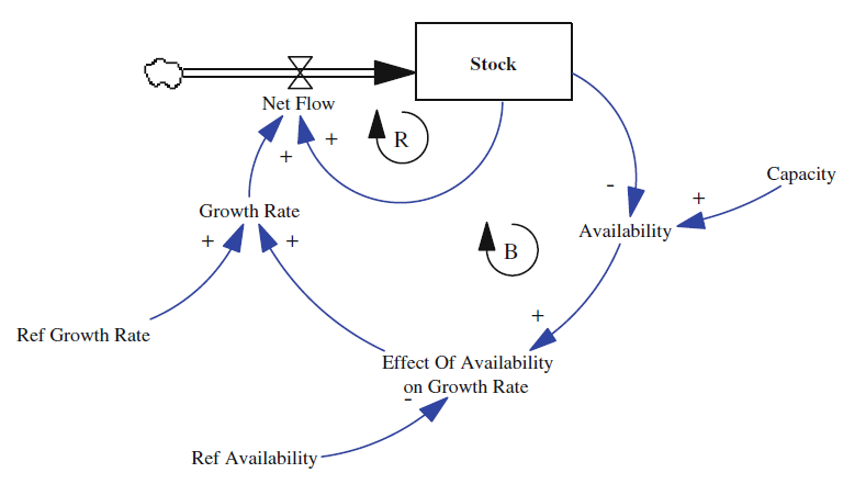
where stock has one inflow with an initial value of 100

\(Stock=\int_{100}^n NetFlow\)

and inflow of

\[NetFlow=Stock∗GrowthRate\]

with system capacity ratio of availability

\[Availability=1−\frac{Stock}{Capacity}\]

and a capacity of 10000 (arbitrary) to limit growth when stock equals capacity since availability will be zero

Capacity=10,000

4.2.2 Declare Variables using deSolve

Using the three R libraries, declare stock and auxiliary variables for the simulation including time period and step.

library(deSolve)
library(ggplot2)
library(gridExtra)

START <- 0
FINISH <- 100
STEP <- 0.25
simtime <- seq(START, FINISH, by = STEP)
stocks <- c(sStock = 100)
auxs <- c(aCapacity = 10000, 
          aRef.Availability = 1,
          aRef.GrowthRate = 0.10)

Set the time period and step. Define the stocks and auxiliaries.

4.2.3 Build a Function

The model’s equations are contained within a function called by deSolve by timestep and passes a vector of stocks with sim values and a vector of auxiliaries. These values are evaluated from the equations (above). The variable dS_dt is an integral. The data frame sModel is created and the first few lines are displayed.

# Create the function
model <- function(time, stocks, auxs){
  with(as.list(c(stocks, auxs)),{
    aAvailability <- 1 - sStock / aCapacity
    aEffect <- aAvailability / aRef.Availability
    aGrowth.Rate <- aRef.GrowthRate * aEffect
    fNet.Flow <- sStock * aGrowth.Rate
    dS_dt <- fNet.Flow
    return(list(c(dS_dt), NetFlow = fNet.Flow,
                GrowthRate = aGrowth.Rate, 
                Effect = aEffect,
                Availability = aAvailability))
  })
}

 Create the data frame

sModel <- data.frame(ode(y = stocks, times = simtime, func = model,
                    parms = auxs, method = "euler"))

head(sModel)

##   time   sStock  NetFlow GrowthRate    Effect Availability
## 1 0.00 100.0000  9.90000 0.09900000 0.9900000    0.9900000
## 2 0.25 102.4750 10.14249 0.09897525 0.9897525    0.9897525
## 3 0.50 105.0106 10.39079 0.09894989 0.9894989    0.9894989
## 4 0.75 107.6083 10.64504 0.09892392 0.9892392    0.9892392
## 5 1.00 110.2696 10.90536 0.09889730 0.9889730    0.9889730
## 6 1.25 112.9959 11.17191 0.09887004 0.9887004    0.9887004

# Run the following snippet to enable `multiplot`
multiplot <- function(..., plotlist=NULL, file, cols=1, layout=NULL) {

  # Make a list from the ... arguments and plotlist
  plots <- c(list(...), plotlist)

  numPlots = length(plots)

  # If layout is NULL, then use 'cols' to determine layout
  if (is.null(layout)) {
    # Make the panel
    # ncol: Number of columns of plots
    # nrow: Number of rows needed, calculated from # of cols
    layout <- matrix(seq(1, cols * ceiling(numPlots/cols)),
                    ncol = cols, nrow = ceiling(numPlots/cols))
  }

 if (numPlots==1) {
    print(plots[[1]])

  } else {
    # Set up the page
    grid.newpage()
    pushViewport(viewport(layout = grid.layout(nrow(layout), ncol(layout))))

    # Make each plot, in the correct location
    for (i in 1:numPlots) {
      # Get the i,j matrix positions of the regions that contain this subplot
      matchidx <- as.data.frame(which(layout == i, arr.ind = TRUE))

      print(plots[[i]], vp = viewport(layout.pos.row = matchidx$row,
                                      layout.pos.col = matchidx$col))
    }
  }
}

4.2.4 Visualize the Variables

The data frame sModel is plotted using ggplot2 and a separate multiplot function to display the following relationships. In the Stock versus Time plot, the classic growth mode is exhibited by an exponential growth to time period 46 followed by a logarithmic growth to 100. The Availability plot mirrors the Stock plot since the resource diminishes as stock increases. The Growth Rate is driven by the effect function

\[ EffectofAvailabilityonGrowthRate=f(AvailabilityRefAvailability),\] \[GrowthRate=RefGrowthRate∗EffectofAvailabilityonGrowthRate\]

and follows Availability until it reaches its capacity. Finally, Net Flow drives the Stock value by rising and falling exponentially with the rate of change.

# Plot the outputs using `multiplot`
stockTimePlot <- sModel %>% 
  ggplot() +
  geom_line(aes(time, sStock), color = "purple")

availTimePlot <- sModel %>% 
  ggplot() +
  geom_line(aes(time, Availability), color = "blue")

netflowTimePlot <- sModel %>% 
  ggplot() +
  geom_line(aes(time, NetFlow), color = "red")

growthrateTimePlot <- sModel %>% 
  ggplot() +
  geom_line(aes(time, GrowthRate), color = "green")

multiplot(stockTimePlot, netflowTimePlot, availTimePlot, growthrateTimePlot, cols = 2)

The above model is related to the differential equation formulated by Belgian mathematician Verhulst in 1845 (below) to model population increase with growth rate r and limit K:

\[\frac{dP}{dt}=rP∗(1−\frac{P}{K})\]

This model assumes the capacity to be constant, which is problematic because the stock is consumed over time in most realistic models (Duggan 2016).

4.2.5 Exercise

What happens when the growth rate is increased to 25%? Show the output in a multiplot.

# Change the growth rate to 0.25
auxs <- c(aCapacity = 10000, 
          aRef.Availability = 1,
          aRef.GrowthRate = 0.25)

# Rerun the function
model <- function(time, stocks, auxs){
  with(as.list(c(stocks, auxs)),{
    aAvailability <- 1 - sStock / aCapacity
    aEffect <- aAvailability / aRef.Availability
    aGrowth.Rate <- aRef.GrowthRate * aEffect
    fNet.Flow <- sStock * aGrowth.Rate
    dS_dt <- fNet.Flow
    return(list(c(dS_dt), NetFlow = fNet.Flow,
                GrowthRate = aGrowth.Rate, 
                Effect = aEffect,
                Availability = aAvailability))
  })
}

# Resave the data frame with the updated auxiliaries and function output
sModel <- data.frame(ode(y = stocks, times = simtime, func = model,
                    parms = auxs, method = "euler"))

# Run `multiplot`
stockTimePlot <- sModel %>% 
  ggplot() +
  geom_line(aes(time, sStock), color = "purple")

availTimePlot <- sModel %>% 
  ggplot() +
  geom_line(aes(time, Availability), color = "blue")

netflowTimePlot <- sModel %>% 
  ggplot() +
  geom_line(aes(time, NetFlow), color = "red")

growthrateTimePlot <- sModel %>% 
  ggplot() +
  geom_line(aes(time, GrowthRate), color = "green")

multiplot(stockTimePlot, netflowTimePlot, availTimePlot, growthrateTimePlot, cols = 2)

4.3 Modeling Constraints—A Non-renewable Stock

Many systems modeled with system dynamics methods involve non-renewable stocks, which are stocks that when depleted cause another stock’s value to decline. The model below depicts how oil well growth, capital, is dependent on the availability of oil, the resource. As capital grows so does the amount of oil extracted. This process has several loops.

Limits to growth for capital, constrained by a non-renewable resource

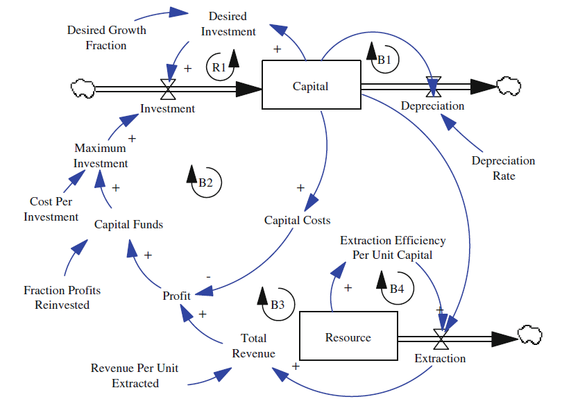
There are five loops in the oil well model of varying types. The positive feedback loop R1 is driven by a desired investment in the capital, the oil wells, whose growth is determined by the growth fraction. Growth is measured by the number of oil wells; more wells equates to more extraction, capital, investment, and profit. The negative feedback loop, B1, accounts for the capital depreciation rate. Over time oil well equipment will need repairs or replacement thus driving depreciation. In the negative feedback loop B2, oil well equipment purchase (startup) costs are driven by the total revenue, amount of reinvestments, profit, and capital costs. More capital results in more oil extraction. However, more investments in capital reduces profits and lower available investments. The negative feedback loops B3 and B4 describe the final aspect of the model, the non-renewable resource oil. As extraction increases with capital, the resource eventually decreases along with extraction efficiency and rate. Efficiency is reduced due to the lack of natural pressure pushing the oil to the surface.

4.3.1 Equations

The capital stock has an initial value of 5 and integrates the difference of investments and depreciation (constant 5%).

\[Capital=\int _5^n Investments∗Depreciation\]

\[Depreciation=Capital∗DepreciationRate\]

DepreciationRate=0.05

The amount of desired investment is the product of growth fraction and capital.

\[DesiredInvestment=DesiredGrowthFraction∗Capital\]

\[DesiredGrowthFraction=0.07\]

Growth is limited by the resource since efficiency decreases, which is defined by extraction rate and is important to understanding feedback loops B3 and B4. The plot of resource by efficiency (below) displays this relationship.

\[Resource=\int_n1000−Extraction\]

\[Extraction=Capital∗ExtractionEfficiencyPerUnitCapital\]

With capital costs set at 10% of capital and revenue per unit extracted at 3, the total revenue can be determined and then deducted to attain the profit.

\[TotalRevenue=RevenuePerUnitExtracted∗Extraction\]

\[RevenuePerUnitExtracted=3\]

\[CapitalCosts=Capital∗0.10\]

\[Profit=TotalRevenue−CapitalCosts\]

The maximum capital investment is calculated by allocating \(12\%\) of profits reinvested at a cost of 2 per investment.

\[FractionProfitsReinvested=0.12\]

\[CapitalFunds=Profit∗FractionProfitsReinvested\]

\[CostPerInvestment=2\]

\[MaximumInvestment=CapitalFundsCostPerInvestment\]

The MIN function is applied as a practical verification for maximum possible investment value so as to not exceed a particular goal.

\[Investment=MIN(DesiredInvestment,MaximumInvestment)\]

The model is initialized with a time period and step along with stocks and auxiliary values and rates.

# Set the time period and step
START <- 0
FINISH <- 200
STEP <- 0.25

# Set the stocks and auxiliaries
simtime <- seq(START, FINISH, by = STEP)
stocks <- c(sCapital = 5, sResource = 1000)
auxs <- c(aDesired.Growth = 0.07,
          aDepreciation = 0.05,
          aCost.Per.Investment = 2.00,
          aFraction.Reinvested = 0.12,
          aRevenue.Per.Unit = 3.00)

The approxfun() function interpolates input and output vectors (resource and extraction) in order to “linearize” the new function’s output, extraction efficiency per unit capital:

ExtractionEfficiencyPerUnitCapital=

Resource	Efficiency
1000	1.0
900	0.99
800	0.98
700	0.96
600	0.92
500	0.85
400	0.75
300	0.63
200	0.45
100	0.25
0	0

# Set the x and y vectors for linearization by the `approxfun` command
x.Resource <- seq(0, 1000, by = 100)
y.Efficiency <- c(0, 0.25, 0.45, 0.63, 0.75, 0.85, 0.92, 0.96, 0.98, 0.99, 1.0)

func.Efficiency <- approxfun(x = x.Resource,
                             y = y.Efficiency,
                             method = "linear",
                             yleft = 0, yright = 1.0)

plot(x.Resource, y.Efficiency)

4.3.2 Function

Given the previous equations and functions, the model’s function is constructed and the ode function called to create a data frame of the output.

# Create the function for the model and the list to return for output
model <- function(time, stocks, auxs){
  with(as.list(c(stocks, auxs)), {
    aExtr.Efficiency <- func.Efficiency(sResource)
    fExtraction <- aExtr.Efficiency * sCapital
    aTotal.Revenue <- aRevenue.Per.Unit * fExtraction
    aCapital.Costs <- sCapital * 0.10
    aProfit <- aTotal.Revenue - aCapital.Costs
    aCapital.Funds <- aFraction.Reinvested * aProfit
    aMaximum.Investment <- aCapital.Funds / aCost.Per.Investment
    aDesired.Investment <- sCapital * aDesired.Growth
    fInvestment <- min(aMaximum.Investment,
                       aDesired.Investment)
    fDepreciation <- sCapital * aDepreciation
    dS_dt <- fInvestment - fDepreciation
    dR_dt <- -fExtraction
    
    return(list(c(dS_dt, dR_dt),
                CapitalCosts = aCapital.Costs,
                Capital = sCapital,
                DesiredInvestment = aDesired.Investment,
                MaximumInvestment = aMaximum.Investment,
                Investment = fInvestment,
                Depreciation = fDepreciation,
                Extraction = fExtraction))
  })
}

# Create the data frame to use for visualizations
nonNewModel <- data.frame(ode(y = stocks, times = simtime, func = model,
                    parms = auxs, method = "euler"))

4.3.3 Outputs

Inspecting the plot generated below depicting extraction, capital, resources, and depreciation shows the relationships of the stocks and flows. Exponential extraction rates precedes capital while reducing the resources, increasing investments (black dashed line) and capital depreciation. Ultimately the resource becomes too expensive to extract as does the capital overhead causing capital and profits to decline.

# Plot the output using `multiplot`
extraction <- nonNewModel %>% 
  ggplot() +
  geom_line(aes(time, Extraction), color = "orange") +
  ylab("Extraction Rate") +
  xlab("Year")

capital <- nonNewModel %>% 
  ggplot() +
  geom_line(aes(time, sCapital), color = "red") +
  ylab("Capital") +
  xlab("Year")

resources <- nonNewModel %>% 
  ggplot() +
  geom_line(aes(time, sResource), color = "purple") +
  ylab("Resource") +
  xlab("Year")

depreciation <- nonNewModel %>% 
  ggplot() +
  geom_line(aes(time, Depreciation), color = "green") +
  geom_line(aes(time, Investment), linetype = "dashed", size = 0.75) +
  ylab("Depreciation") +
  xlab("Year")

## Warning: Using `size` aesthetic for lines was deprecated in ggplot2 3.4.0.
## ℹ Please use `linewidth` instead.
## This warning is displayed once every 8 hours.
## Call `lifecycle::last_lifecycle_warnings()` to see where this warning was
## generated.

multiplot(extraction, capital, resources, depreciation, cols = 2)

4.3.4 Maximum Values

For this scenario, the years during which maximum capital and extraction rates occur are calculated. These are particularly useful when conveying strengths and liabilities.

# Find the time (year) in which the maximum capital and extraction rate are realized
nonNewModel[which.max(nonNewModel$sCapital), "time"]

## [1] 87

## [1] 87
nonNewModel[which.max(nonNewModel$Extraction), "time"]

## [1] 64.25

4.3.5 Exercise

Increase the capital depreciation to 25% and plot the output using multiplot. Explain the results.

# Change the aDepreciation from 0.05 to 0.25
auxs <- c(aDesired.Growth = 0.07,
          aDepreciation = 0.25,
          aCost.Per.Investment = 2.00,
          aFraction.Reinvested = 0.12,
          aRevenue.Per.Unit = 3.00)

# Run the `model2` function
model2 <- function(time, stocks, auxs){
  with(as.list(c(stocks, auxs)), {
    aExtr.Efficiency <- func.Efficiency(sResource)
    fExtraction <- aExtr.Efficiency * sCapital
    aTotal.Revenue <- aRevenue.Per.Unit * fExtraction
    aCapital.Costs <- sCapital * 0.10
    aProfit <- aTotal.Revenue - aCapital.Costs
    aCapital.Funds <- aFraction.Reinvested * aProfit
    aMaximum.Investment <- aCapital.Funds / aCost.Per.Investment
    aDesired.Investment <- sCapital * aDesired.Growth
    fInvestment <- min(aMaximum.Investment,
                       aDesired.Investment)
    fDepreciation <- sCapital * aDepreciation
    dS_dt <- fInvestment - fDepreciation
    dR_dt <- -fExtraction
    
    return(list(c(dS_dt, dR_dt),
                CapitalCosts = aCapital.Costs,
                Capital = sCapital,
                DesiredInvestment = aDesired.Investment,
                MaximumInvestment = aMaximum.Investment,
                Investment = fInvestment,
                Depreciation = fDepreciation,
                Extraction = fExtraction))
  })
}

# Run the `data.frame` command
nonNewModel2 <- data.frame(ode(y = stocks, times = simtime, func = model2,
                    parms = auxs, method = "euler"))

# Run `ggplot` for each variable and `multiplot` for the visualization
extraction <- nonNewModel2 %>% 
  ggplot() +
  geom_line(aes(time, Extraction), color = "orange") +
  ylab("Extraction Rate") +
  xlab("Year")

capital <- nonNewModel2 %>% 
  ggplot() +
  geom_line(aes(time, sCapital), color = "red") +
  ylab("Capital") +
  xlab("Year")

resources <- nonNewModel2 %>% 
  ggplot() +
  geom_line(aes(time, sResource), color = "purple") +
  ylab("Resource") +
  xlab("Year")

depreciation <- nonNewModel2 %>% 
  ggplot() +
  geom_line(aes(time, Depreciation), color = "green") +
  geom_line(aes(time, Investment), linetype = "dashed", size = 0.75) +
  ylab("Depreciation") +
  xlab("Year")

multiplot(extraction, capital, resources, depreciation, cols = 2)

4.3.6 Creating Scenarios: Effect of Growth Rate on Results

System dynamics modeling often allows users to investigate multiple secarios for consideration. Using the rbind() function to append data sets, a range of growth rates is then displayed in the graph below. Given the outputs of the model (above), the changes to capital, extraction rate, and investments becomes apparent. Typically, the more aggressive the growth rate the more rapid the extraction and subsequently the consumption of the resource.

# Change the aDepreciation back to 0.05
auxs <- c(aDesired.Growth = 0.07,
          aDepreciation = 0.05,
          aCost.Per.Investment = 2.00,
          aFraction.Reinvested = 0.12,
          aRevenue.Per.Unit = 3.00)

# Function to automate `rbind()` below. The function formals include `stocks`, `simtime`, `model`, and `auxs`, which were defined in the arguments of the previous data frame command. 

scenarios <- function(GRate, n, stocks, simtime, model, auxs, step = 0.01) {
    vec <- seq(GRate, by = step, length.out = n)
    base <- data.frame()
    for (i in 1:length(vec)) {
        auxs["aDesired.Growth"] <- vec[i]
        temp <- data.frame(ode(y = stocks, times = simtime, func = model, parms = auxs, method = "euler"))
        temp$GR <- paste0("GR = ",100*vec[i],"%")
        base <- rbind(base,temp)
    }
    return(base)
}

base <- scenarios(0.05, 7, stocks, simtime, model, auxs)

# Plot the scenarios
base %>% 
  ggplot() +
  geom_line(aes(time, Extraction, color = base$GR)) +
  xlab("Year") +
  ylab("Extraction Rate") +
  theme(legend.position = "bottom") +
  guides(color = guide_legend(title = NULL)) +
  ggtitle("Growth Rate Scenarios")

## Warning: Use of `base$GR` is discouraged.
## ℹ Use `GR` instead.

4.3.7 Exercise

Plot a set of six growth rate scenarios from two to seven percent. Identify the year the maximum extraction rate occurs.

# Generate the growth rate scenarios
base <- scenarios(0.02, 6, stocks, simtime, model, auxs)

# Plot the scenarios
base %>% 
  ggplot() +
  geom_line(aes(time, Extraction, color = base$GR)) +
  xlab("Year") +
  ylab("Extraction Rate") +
  theme(legend.position = "bottom") +
  guides(color = guide_legend(title = NULL)) +
  ggtitle("Growth Rate Scenarios")

## Warning: Use of `base$GR` is discouraged.
## ℹ Use `GR` instead.

# Determine the year maximum extraction rate occurs
base[which.max(base$Extraction), "time"]

## [1] 64.25

It is important to acknowledge that this model is paramount in a variety of industries where growth has to be considered based on the available resources, whether that be oil, patients, or customers where several independent variables act upon a dependent variable. Given the toy instance described above, it is easy to imagine the complexity of a more realistic and pragmatic model with dozens of stocks and flows.

References

Duggan, Jim. 2016. System Dynamics Modeling with R: Lecture Notes in Social Networks.

Forrester, Jay W. 1968. Principles of Systems. Cambridge: Wright-Allen Press, Inc.

System Dynamics Society. 2017. “Origin of System Dynamics.” Accessed August 2. http://www.systemdynamics.org/DL-IntroSysDyn/origin.htm.