9 Taller Redes Neuronales
9.1 Carge de bibliotecas
library(neuralnet)  # regression

library(nnet) # classification

library(NeuralNetTools)

library(plyr)

library(kableExtra)
9.2 Carga de Datos
library(readr)
Startups <- read_csv("/media/rpalma/OS/AAA_Datos/2020/Posgrado/Di3/Datasets/50 Start Ups/50_Startups_LAC.csv")
## Parsed with column specification:
## cols(
## R_D_Spend = col_double(),
## POM = col_double(),
## Logist_Market = col_double(),
## Pais = col_character(),
## Profit = col_double(),
## Supervivencia = col_double()
## )Categoric <- read_csv("/media/rpalma/OS/AAA_Datos/2020/Posgrado/Di3/Datasets/50 Start Ups/50_Startups_Categoric_LAC.csv")## Parsed with column specification:
## cols(
## R_D_Spend = col_double(),
## POM = col_double(),
## Logist_Market = col_double(),
## Pais = col_character(),
## Profit = col_double(),
## Supervivencia = col_character()
## )9.3 Tratamiento de variables categóricas
tabla1 <- table(Categoric$Pais)
tabla2 <- table(Categoric$Supervivencia)
tabla3 <- table(Categoric$Pais,Categoric$Supervivencia)plot(tabla1, col=c("red","green","blue"))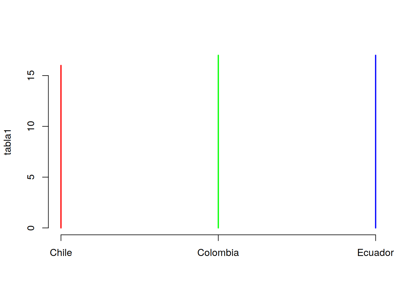
plot(tabla2, col=c("red","green","blue"))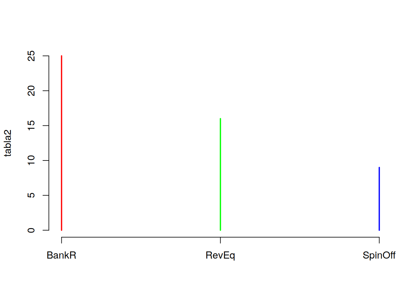
plot(tabla3, col=c("red","green","blue"))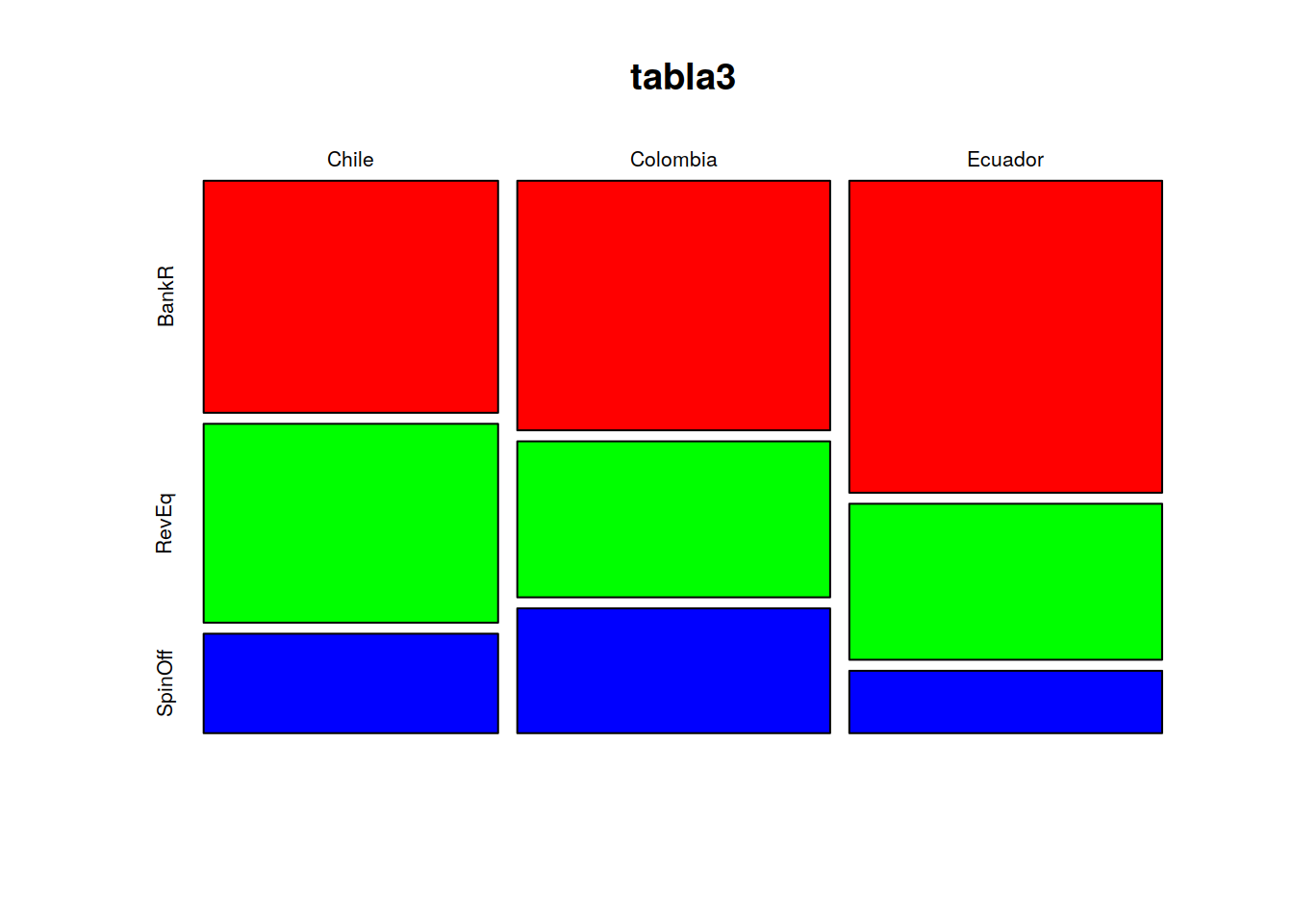
9.4 Histogramas superpuestos
ind_1 <- which(Categoric$Pais=="Colombia")
p1 <- as.matrix(Categoric[ind_1,5])

ind_2 <- which(Categoric$Pais=="Ecuador")
p2 <- as.matrix(Categoric[ind_2,5])

ind_3 <- which(Categoric$Pais=="Chile")
p3 <- as.matrix(Categoric[ind_3,5])
hp1 <- hist(p1)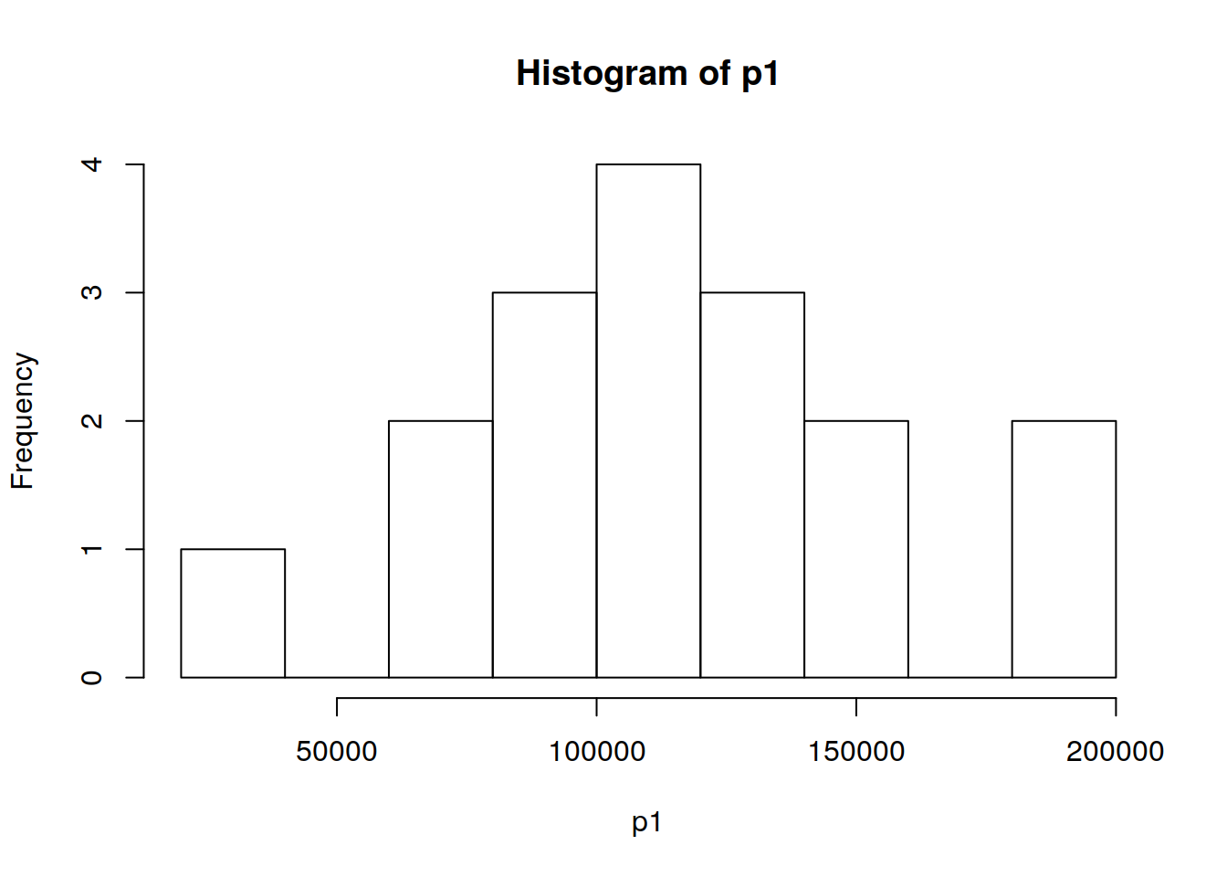
hp2 <- hist(p2)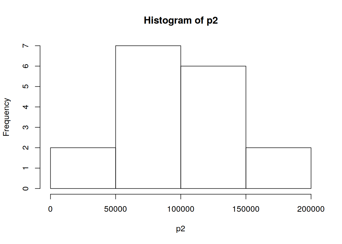
hp3 <- hist(p3)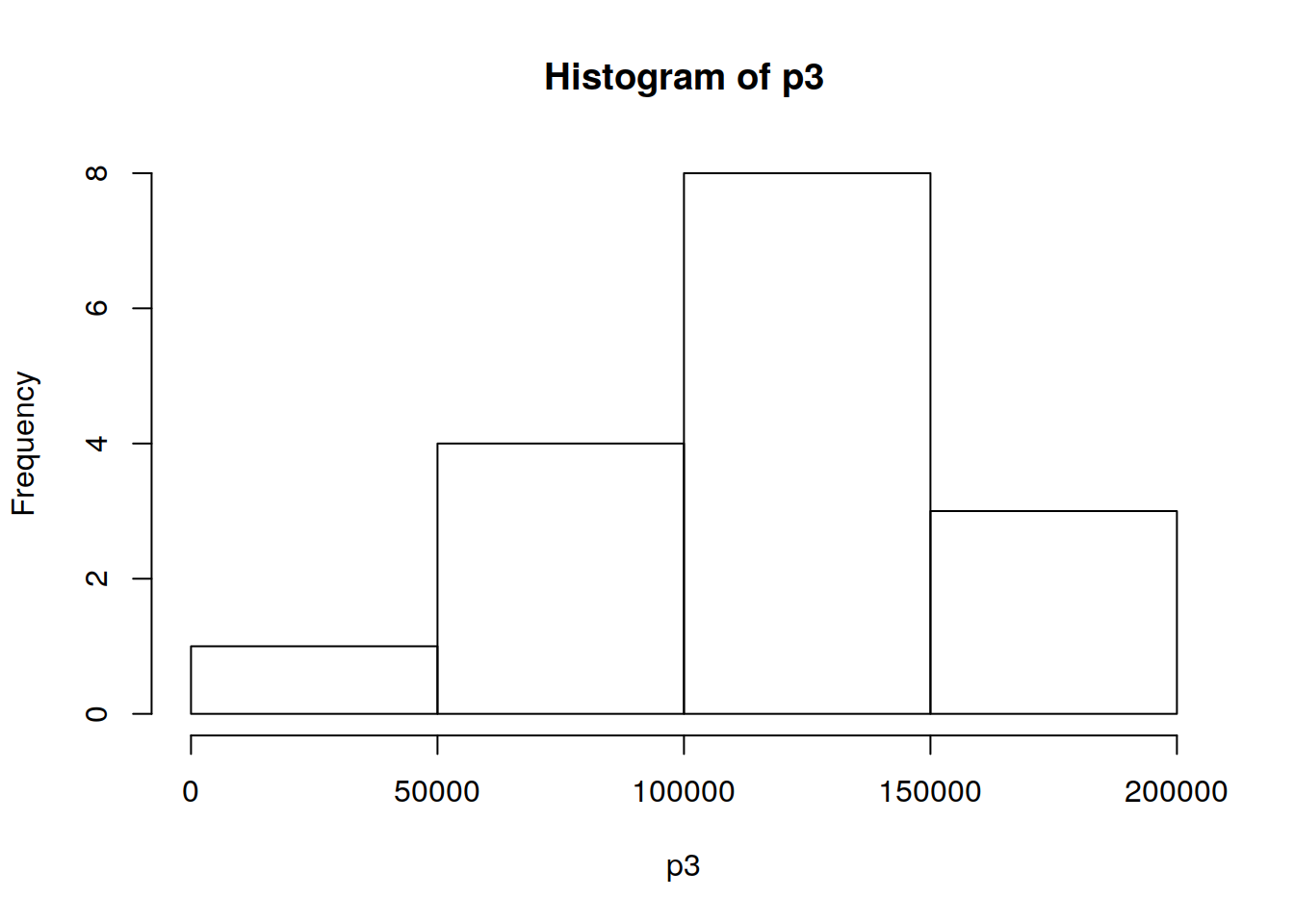
par(mfrow=c(3,1))
plot( hp1, col=rgb(0,0,1,1/4), xlim=c(30000,200000),ylim=c(0,5),main="Ecuador")
plot( hp2, col=rgb(1,0,0,1/4),xlim=c(30000,200000),ylim=c(0,10),main="Colombia")
plot( hp3, col=rgb(1,0,0,1/4),xlim=c(30000,200000),ylim=c(0,10),main="Chile") 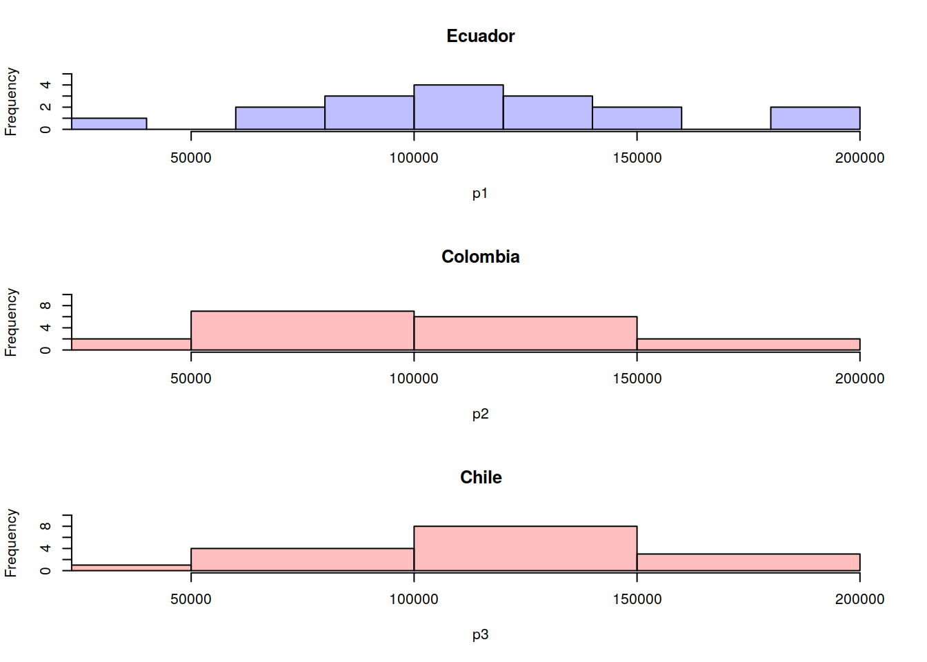
par(mfrow=c(1,3))
plot( hp1, col=rgb(0,0,1,1/4), xlim=c(30000,200000),ylim=c(0,5),main="Ecuador")
plot( hp2, col=rgb(1,0,0,1/4),xlim=c(30000,200000),ylim=c(0,10),main="Colombia")
plot( hp3, col=rgb(1,0,0,1/4),xlim=c(30000,200000),ylim=c(0,10),main="Chile") 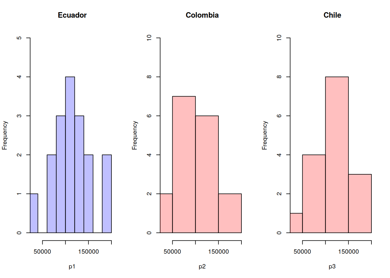
pairs(Categoric[ ,1:3])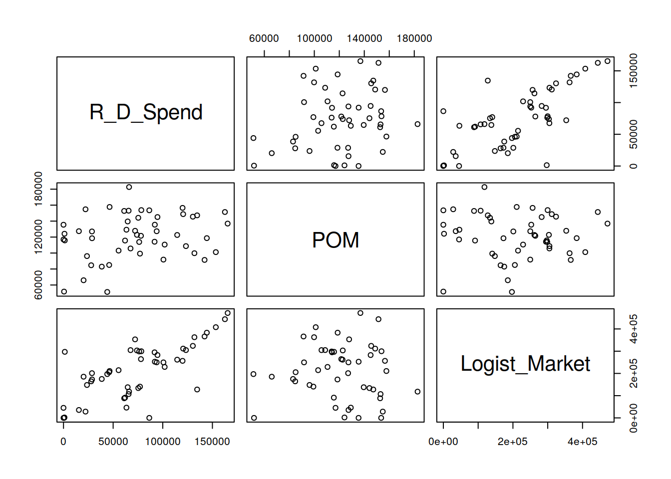
boxplot(Categoric[ ,1:3])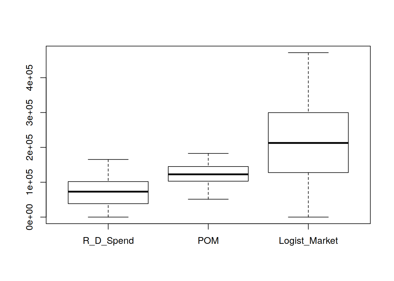
Categoric$Pais <- as.numeric(revalue(Categoric$Pais,
                          c("Colombia"="0", "Ecuador"="1",
                            "Chile"="2")))
9.5 Cuadro de campos categóricos
Categoric$Supervivencia <- as.numeric(revalue(Categoric$Supervivencia,
                          c("BankR"="0", "RevEq"="1",
                            "SpinOff"="2")))
9.6 Profit versus País
plot(Categoric$Pais, Categoric$Profit)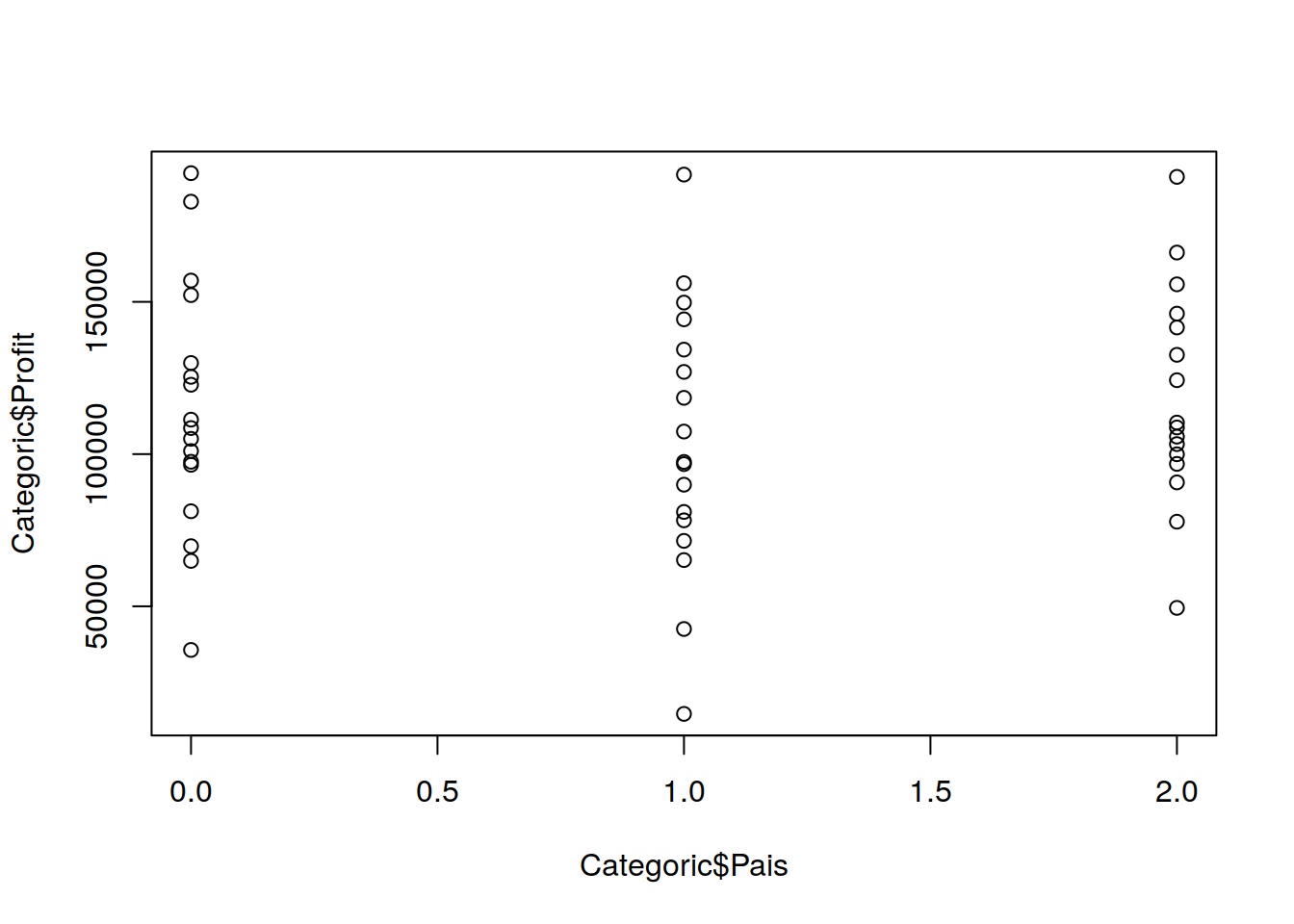
9.7 Visualización de Tablas
Tabla Textual
library(kableExtra)
kable(head(Categoric), "pipe")| R_D_Spend | POM | Logist_Market | Pais | Profit | Supervivencia |
|---|---|---|---|---|---|
| 165349.2 | 136897.80 | 471784.1 | 0 | 192261.8 | 2 |
| 162597.7 | 151377.59 | 443898.5 | 1 | 191792.1 | 2 |
| 153441.5 | 101145.55 | 407934.5 | 2 | 191050.4 | 2 |
| 144372.4 | 118671.85 | 383199.6 | 0 | 182902.0 | 2 |
| 142107.3 | 91391.77 | 366168.4 | 2 | 166187.9 | 2 |
| 131876.9 | 99814.71 | 362861.4 | 0 | 156991.1 | 2 |
Tabla Simple
kable(head(Categoric), "simple")| R_D_Spend | POM | Logist_Market | Pais | Profit | Supervivencia |
|---|---|---|---|---|---|
| 165349.2 | 136897.80 | 471784.1 | 0 | 192261.8 | 2 |
| 162597.7 | 151377.59 | 443898.5 | 1 | 191792.1 | 2 |
| 153441.5 | 101145.55 | 407934.5 | 2 | 191050.4 | 2 |
| 144372.4 | 118671.85 | 383199.6 | 0 | 182902.0 | 2 |
| 142107.3 | 91391.77 | 366168.4 | 2 | 166187.9 | 2 |
| 131876.9 | 99814.71 | 362861.4 | 0 | 156991.1 | 2 |
9.8 Normailización
normalize<-function(x){
  return ( (x-min(x))/(max(x)-min(x)))
}

Startups_norm<-as.data.frame(lapply(Categoric,FUN=normalize))
summary(Startups_norm$Profit)
## Min. 1st Qu. Median Mean 3rd Qu. Max.
## 0.0000 0.4249 0.5254 0.5481 0.7044 1.0000Datos Originales y Datos normalizados
head(Categoric$Profit)## [1] 192261.8 191792.1 191050.4 182902.0 166187.9
## [6] 156991.1head(Startups_norm)## R_D_Spend POM Logist_Market Pais
## 1 1.0000000 0.6517439 1.0000000 0.0
## 2 0.9833595 0.7619717 0.9408934 0.5
## 3 0.9279846 0.3795790 0.8646636 1.0
## 4 0.8731364 0.5129984 0.8122351 0.0
## 5 0.8594377 0.3053280 0.7761356 1.0
## 6 0.7975660 0.3694479 0.7691259 0.0
## Profit Supervivencia
## 1 1.0000000 1
## 2 0.9973546 1
## 3 0.9931781 1
## 4 0.9472924 1
## 5 0.8531714 1
## 6 0.8013818 1Muestreo para entrenamento
indice <- sample(2, nrow(Startups_norm), replace = TRUE, prob = c(0.7,0.3))
startups_train <- Startups_norm[indice==1,]
startups_test  <- Startups_norm[indice==2,]
9.9 Modelo de Neural Net
attach(Categoric)

startups_model <- neuralnet(Profit~R_D_Spend+ POM + Logist_Market + Pais
, data = startups_train)
str(startups_model)
## List of 14
## $ call : language neuralnet(formula = Profit ~ R_D_Spend + POM + Logist_Market + Pais, data = startups_train)
## $ response : num [1:26, 1] 0.997 0.947 0.853 0.796 0.774 ...
## ..- attr(*, "dimnames")=List of 2
## .. ..$ : chr [1:26] "2" "4" "5" "7" ...
## .. ..$ : chr "Profit"
## $ covariate : num [1:26, 1:4] 0.983 0.873 0.859 0.814 0.729 ...
## ..- attr(*, "dimnames")=List of 2
## .. ..$ : chr [1:26] "2" "4" "5" "7" ...
## .. ..$ : chr [1:4] "R_D_Spend" "POM" "Logist_Market" "Pais"
## $ model.list :List of 2
## ..$ response : chr "Profit"
## ..$ variables: chr [1:4] "R_D_Spend" "POM" "Logist_Market" "Pais"
## $ err.fct :function (x, y)
## ..- attr(*, "type")= chr "sse"
## $ act.fct :function (x)
## ..- attr(*, "type")= chr "logistic"
## $ linear.output : logi TRUE
## $ data :'data.frame': 26 obs. of 6 variables:
## ..$ R_D_Spend : num [1:26] 0.983 0.873 0.859 0.814 0.729 ...
## ..$ POM : num [1:26] 0.762 0.513 0.305 0.73 0.742 ...
## ..$ Logist_Market: num [1:26] 0.941 0.812 0.776 0.271 0.66 ...
## ..$ Pais : num [1:26] 0.5 0 1 0.5 0 1 0.5 1 0.5 0.5 ...
## ..$ Profit : num [1:26] 0.997 0.947 0.853 0.796 0.774 ...
## ..$ Supervivencia: num [1:26] 1 1 1 1 1 0.5 0.5 0.5 0.5 0.5 ...
## $ exclude : NULL
## $ net.result :List of 1
## ..$ : num [1:26, 1] 0.935 0.909 0.886 0.807 0.81 ...
## .. ..- attr(*, "dimnames")=List of 2
## .. .. ..$ : chr [1:26] "2" "4" "5" "7" ...
## .. .. ..$ : NULL
## $ weights :List of 1
## ..$ :List of 2
## .. ..$ : num [1:5, 1] -1.438 3.448 -0.419 0.556 -0.2
## .. ..$ : num [1:2, 1] 0.087 0.956
## $ generalized.weights:List of 1
## ..$ : num [1:26, 1:4] 5.43 4.8 4.49 3.94 3.95 ...
## .. ..- attr(*, "dimnames")=List of 2
## .. .. ..$ : chr [1:26] "2" "4" "5" "7" ...
## .. .. ..$ : NULL
## $ startweights :List of 1
## ..$ :List of 2
## .. ..$ : num [1:5, 1] 0.5926 -0.7423 -0.0559 2.1104 -0.6281
## .. ..$ : num [1:2, 1] 0.678 1.606
## $ result.matrix : num [1:10, 1] 0.01743 0.00727 93 -1.43786 3.44781 ...
## ..- attr(*, "dimnames")=List of 2
## .. ..$ : chr [1:10] "error" "reached.threshold" "steps" "Intercept.to.1layhid1" ...
## .. ..$ : NULL
## - attr(*, "class")= chr "nn"9.10 Ploteo de la red Neuronal
plot(startups_model, rep = "best")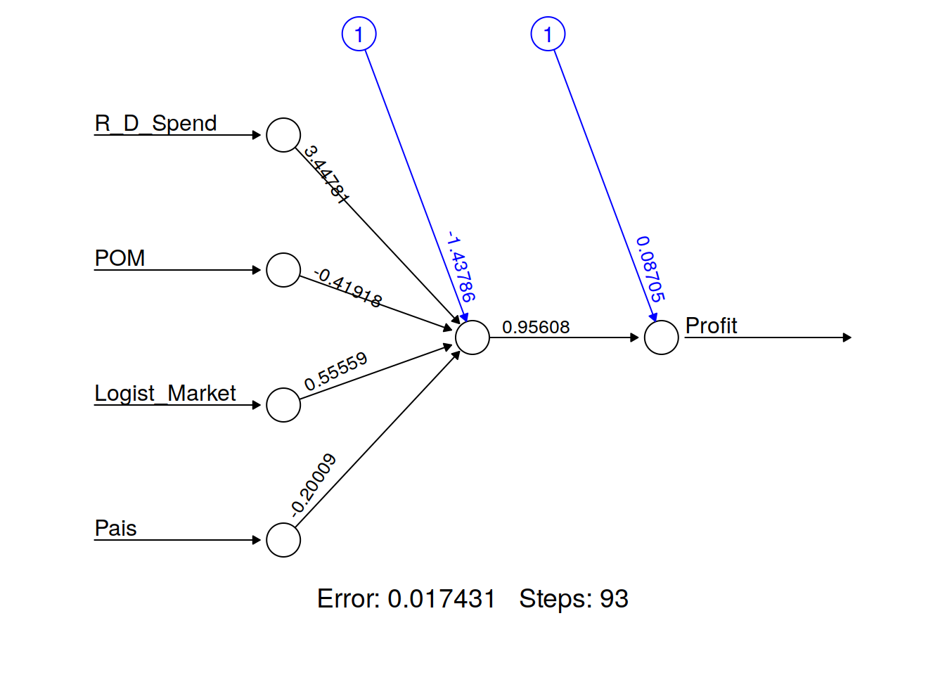
9.11 Ploteo de la red proporcional
Esto me indica cuales son los KPI
par(mar = numeric(4), family = 'serif')
plotnet(startups_model, alpha = 0.6)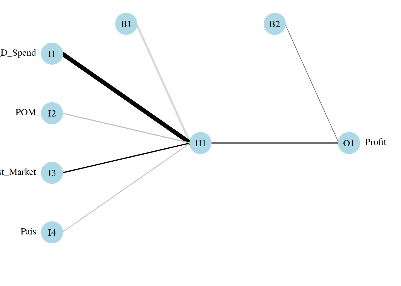
9.11.1 Evaluación de la performance del modelo
model_results <- compute(startups_model,startups_test[1:4])
predicted_profit <- model_results$net.result
9.12 Predicted profit Vs Actual profit of test data.
cor(predicted_profit,startups_test$Profit)## [,1]
## [1,] 0.95229069.13 Desnormalización de los resultados
Dado que hicimos la predicciones con los datos normalizados, ahora deberemos des-normalizarlos
str_max <- max(Startups$Profit)
str_min <- min(Startups$Profit)

unnormalize <- function(x, min, max) {
  return( (max - min)*x + min )
}

ActualProfit_pred <- unnormalize(predicted_profit,str_min,str_max)
head(ActualProfit_pred)
## [,1]
## 1 184342.2
## 3 177499.6
## 6 171030.0
## 8 159389.2
## 10 160917.4
## 12 144564.59.14 Mejoramiento de la performance del modelo
Es posible mejorar la performance con el agregado de más capas ocultas.
Startups_model2 <- neuralnet(Profit~R_D_Spend+ POM + Logist_Market + Pais
, data = startups_train, hidden = 2)
plot(Startups_model2 ,rep = "best")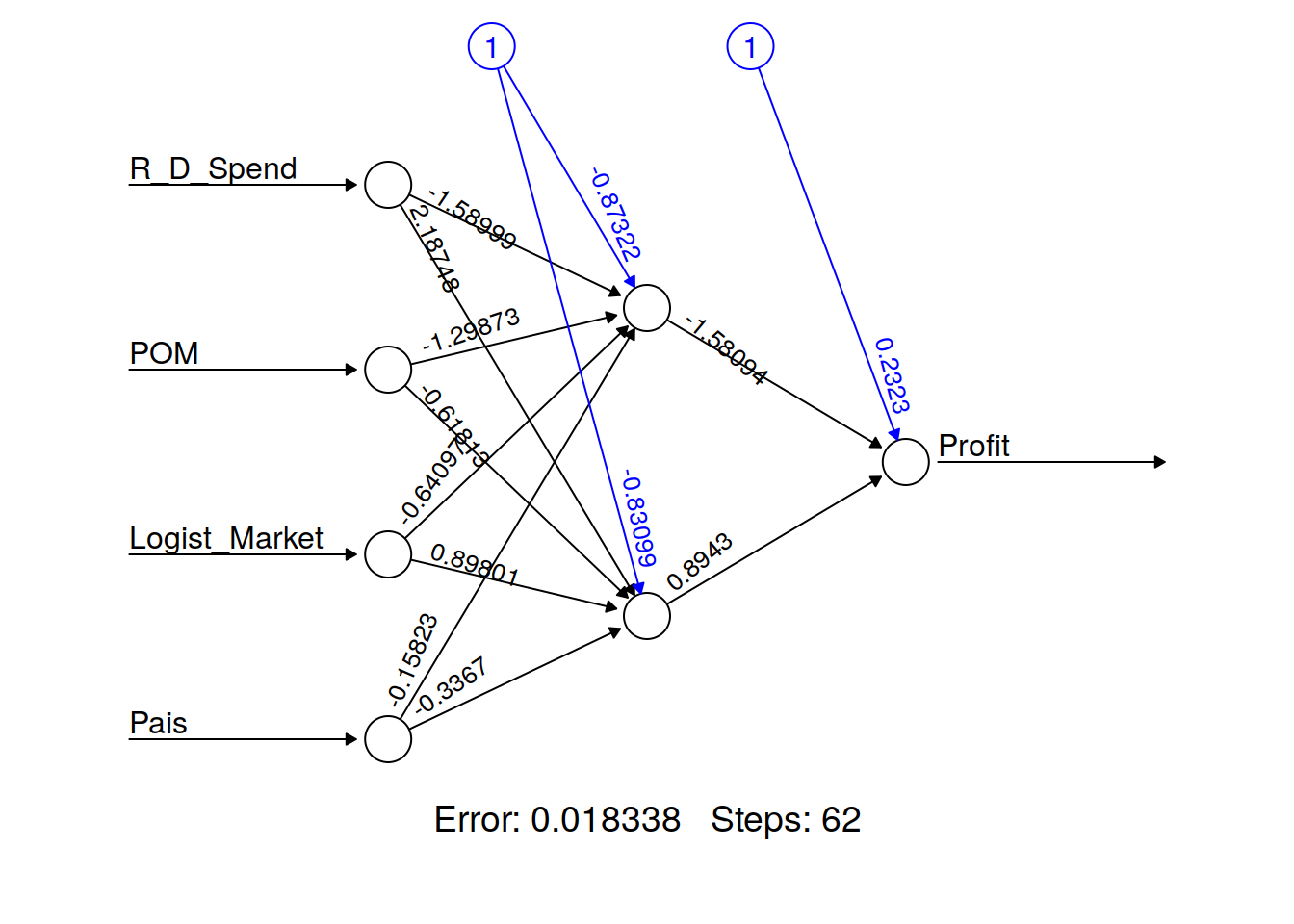
9.15 Performance del modelo mejorado
model_results2<-compute(Startups_model2,startups_test[1:4])
predicted_Profit2<-model_results2$net.result
cor(predicted_Profit2,startups_test$Profit)
## [,1]
## [1,] 0.94281869.16 Modelo Mejorado KPI
par(mar = numeric(4), family = 'serif')
plotnet(Startups_model2, alpha = 0.6)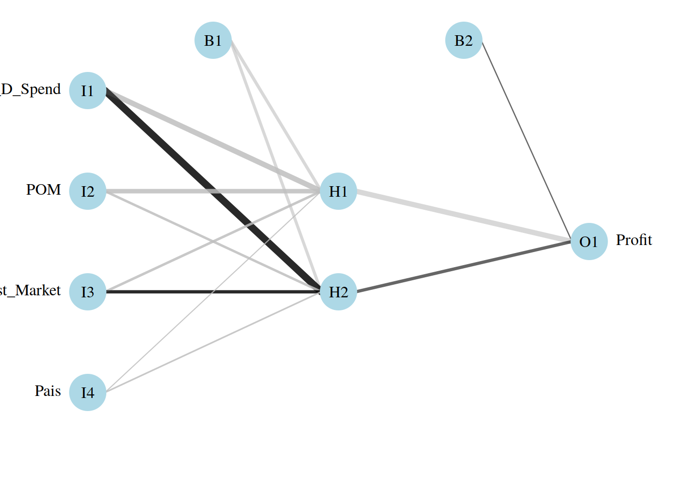
9.17 Neural Net Clasificación
Armamos el dataset de datos a clasificar
library(nnet)

supervivencia <- as.factor(Categoric$Supervivencia)
R_D_Spend <- as.matrix(Categoric$R_D_Spend)
POM <- as.matrix(Categoric$POM)
Logist_Market <- as.matrix(Categoric$Logist_Market)
Clasificar <- data.frame (supervivencia,R_D_Spend,POM,Logist_Market)
9.18 Muestreo
indice <- sample(2, nrow(Clasificar), replace = TRUE, prob = c(0.7,0.3))

clasificar_train <- Startups_norm[indice==1,]
clasificar_test  <- Startups_norm[indice==2,]

supervivientes_clasificados <- factor(clasificar_train$Supervivencia)
Entrenamiento de nnet como clasificador
supervivientes_train<-nnet(supervivientes_clasificados~clasificar_train$R_D_Spend + clasificar_train$POM+ clasificar_train$Logist_Market ,data=clasificar_train,size=5, decay=5e-4, maxit=2000)## # weights: 38
## initial value 33.902626
## iter 10 value 8.725337
## iter 20 value 3.961923
## iter 30 value 2.486946
## iter 40 value 1.878157
## iter 50 value 1.480637
## iter 60 value 1.378036
## iter 70 value 1.304077
## iter 80 value 1.252581
## iter 90 value 1.229374
## iter 100 value 1.211815
## iter 110 value 1.195886
## iter 120 value 1.187665
## iter 130 value 1.183899
## iter 140 value 1.180618
## iter 150 value 1.176144
## iter 160 value 1.173408
## iter 170 value 1.172258
## iter 180 value 1.170433
## iter 190 value 1.169332
## iter 200 value 1.166716
## iter 210 value 1.164242
## iter 220 value 1.163139
## iter 230 value 1.161066
## iter 240 value 1.160280
## iter 250 value 1.159733
## iter 260 value 1.159332
## iter 270 value 1.158817
## iter 280 value 1.158632
## iter 290 value 1.157832
## iter 300 value 1.156969
## iter 310 value 1.156118
## iter 320 value 1.155847
## iter 330 value 1.155571
## iter 340 value 1.154717
## iter 350 value 1.154154
## iter 360 value 1.153444
## iter 370 value 1.152567
## iter 380 value 1.152300
## iter 390 value 1.152219
## iter 400 value 1.152196
## iter 410 value 1.152148
## iter 420 value 1.152125
## iter 430 value 1.152108
## iter 440 value 1.152100
## iter 450 value 1.152095
## iter 460 value 1.152090
## final value 1.152088
## converged9.19 Visualización del clasificador
plotnet(supervivientes_train, alpha = 0.6)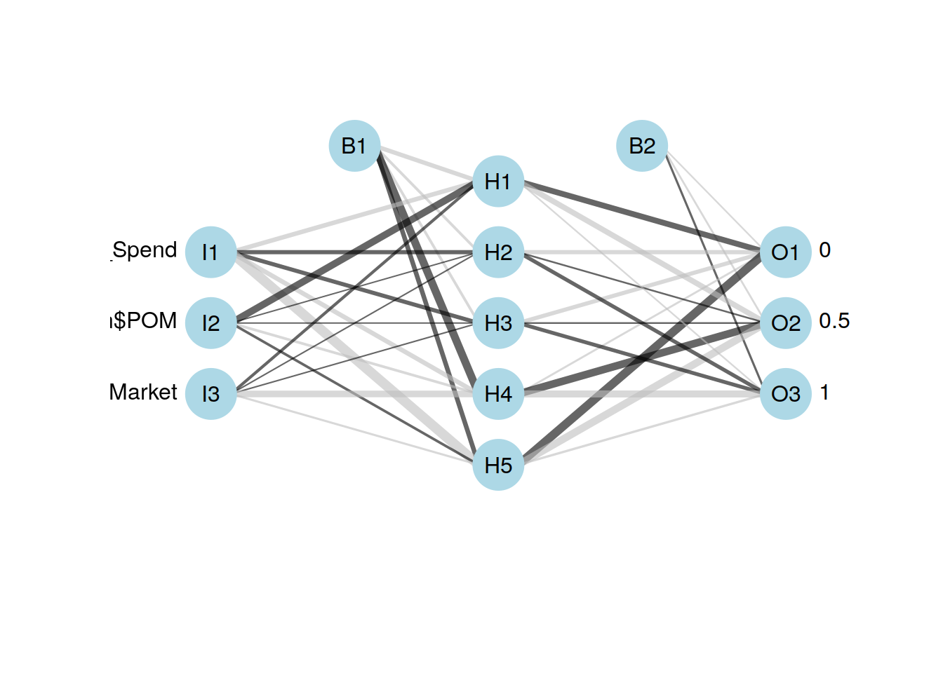
9.20 Aramdos de set de entrenamiento y de predicción
https://stackoverrun.com/es/q/3338607
crs\(nnet <- nnet(as.factor(Target) ~ ., data=crs\)dataset[crs\(sample,c(crs\)input, crs$target)], size=10, skip=TRUE, MaxNWts=10000, trace=FALSE, maxit=100)